Variational Estimation for Multidimensional Item Response Theory Using VEMIRT
Source:vignettes/VEMIRT.Rmd
VEMIRT.RmdIntroduction
In this tutorial, we illustrate how to conduct multidimensional item
response theory (MIRT) analysis of multidimensional two parameter
logistic (M2PL) and multidimensional three parameter logistic (M3PL)
models, and differential item functioning (DIF) analysis of M2PL models
using the VEMIRT package in R, which can be
installed with
if (!require(devtools)) install.packages("devtools")
devtools::install_github("MAP-LAB-UW/VEMIRT", build_vignettes = T)
torch::install_torch()
The package requires a C++ compiler to work properly, and users are referred to https://github.com/MAP-LAB-UW/VEMIRT for more information.
Most functions are based on the Gaussian variational expectation-maximization (GVEM) algorithm, which is applicable for high-dimensional latent traits.
Data Input
Data required for analysis are summarized below:
| Analysis | Item Responses | Loading Indicator | Group Membership |
|---|---|---|---|
| Exploratory Factor Analysis | \checkmark | ||
| Confirmatory Factor Analysis | \checkmark | \checkmark | |
| Differential Item Functioning | \checkmark | \checkmark | \checkmark |
Here we take dataset D2PL_data as an example. This
simulated dataset is for DIF 2PL analysis. Responses should be an N by J
binary matrix, where N and J are the numbers of respondents and items
respectively. Currently, all DIF functions and C2PL_iw2
allow responses to have missing data, which should be coded as
NA. In this example, there are N=1500 respondents and J=20 items.
head(D2PL_data$data)
#>      [,1] [,2] [,3] [,4] [,5] [,6] [,7] [,8] [,9] [,10] [,11] [,12] [,13] [,14] [,15] [,16] [,17] [,18] [,19]
#> [1,]    0    1    0    1    1    0    1    0    0     0     1     0     0     1     0     1     1     1     1
#> [2,]    0    0    0    0    1    0    0    0    0     0     0     0     0     1     0     0     0     0     0
#> [3,]    0    0    0    0    0    0    1    0    0     0     0     0     0     0     0     0     1     0     1
#> [4,]    0    0    1    0    1    0    0    0    0     1     1     1     1     1     1     1     0     1     0
#> [5,]    0    0    0    0    0    0    0    0    0     1     0     0     0     0     0     1     0     0     0
#> [6,]    1    1    1    1    1    0    1    1    1     1     1     1     1     1     1     1     1     1     0
#>      [,20]
#> [1,]     0
#> [2,]     0
#> [3,]     0
#> [4,]     0
#> [5,]     0
#> [6,]     1
CFA and DIF rely on a J by D binary loading indicator matrix specifying latent dimensions each item loads on, where D is the number of latent dimensions. The latent traits have D=2 dimensions here.
D2PL_data$model
#>       [,1] [,2]
#>  [1,]    1    0
#>  [2,]    0    1
#>  [3,]    1    0
#>  [4,]    0    1
#>  [5,]    1    0
#>  [6,]    0    1
#>  [7,]    1    0
#>  [8,]    0    1
#>  [9,]    1    0
#> [10,]    0    1
#> [11,]    1    0
#> [12,]    0    1
#> [13,]    1    0
#> [14,]    0    1
#> [15,]    1    0
#> [16,]    0    1
#> [17,]    1    0
#> [18,]    0    1
#> [19,]    1    0
#> [20,]    0    1
DIF analysis additionally needs a group membership vector of length N, whose elements are integers from 1 to G, where G is the number of groups. There are G=3 groups in this example.
table(D2PL_data$group)
#>
#>   1   2   3
#> 500 500 500
Data Output
All the functions output estimates of item parameters and some other
related parameters. In addition, C2PL_gvem,
C2PL_bs and C2PL_iw2 are able to provide the
standard errors of item parameter estimates.
Exploratory Factor Analysis
Parallel Analysis
Parallel analysis can be conducted to determine the number of
factors. Users can specify the number of simulated datasets, which takes
n.iter = 10 by default.
pa_poly(D2PL_data$data, n.iter = 5)
#> Parallel analysis suggests that the number of factors =  2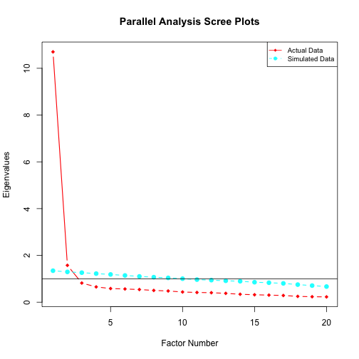
M2PL Model
VEMIRT provides the following functions to conduct EFA
for the M2PL model:
| Function | Description |
|---|---|
E2PL_gvem_rot |
GVEM with post-hoc rotation |
E2PL_gvem_lasso |
GVEM with lasso penalty |
E2PL_gvem_adaptlasso |
GVEM with adaptive lasso penalty |
E2PL_iw |
Importance sampling for GVEM |
Currently these functions do not estimate the standard errors of item
parameters. The following examples use two simulated datasets,
E2PL_data_C1 and E2PL_data_C2, both having
N=1000 respondents, J=30 items and D=3 dimensions, but items load on different
dimensions.
E2PL_gvem_rot needs the item responses and the number of
factors (domain), and applies the promax rotation
(rot = "Promax") by default. Another choice is
rot = "cfQ", which performs the CF-Quartimax rotation.
E2PL_gvem_rot(E2PL_data_C1$data, domain = 3)
#>          a1      a2       a3       b
#> 1   0.10594  1.5952 -0.10845  1.7290
#> 2   1.91968  0.0721 -0.05631 -1.3236
#> 3   0.07972 -0.0394  1.56129 -1.2989
#> 4   0.19942  1.8727 -0.05273 -0.8808
#> 5   1.73784  0.0441 -0.11143 -0.8111
#> 6  -0.05117  0.0230  1.63743  0.1912
#> 7  -0.05174  1.3707 -0.00506 -0.9726
#> 8   1.52949  0.1766 -0.03231  0.4670
#> 9  -0.01529  0.0186  1.42425  1.1823
#> 10  0.04563  1.4053  0.07149  1.0613
#> 11  1.64560 -0.0849  0.06168  0.8636
#> 12  0.08978  0.0130  1.65967 -0.6542
#> 13  0.10412  1.8613  0.09076  0.0380
#> 14  1.42716 -0.1292  0.18454  1.5696
#> 15  0.03152  0.0564  1.78979 -1.3211
#> 16 -0.03327  1.7001  0.17390 -1.9581
#> 17  1.84224 -0.0486 -0.00188  0.5343
#> 18 -0.00405 -0.0918  1.60662  0.5123
#> 19 -0.19546  1.8230 -0.07211  0.1182
#> 20  1.34056 -0.0278  0.07707  0.3125
#> 21  0.14051 -0.0800  1.71112  0.1102
#> 22 -0.06479  1.9194 -0.02918 -0.6766
#> 23  1.55836  0.2900  0.05540  1.0387
#> 24 -0.20321  0.1247  1.59738  0.0535
#> 25  0.04718  1.4758  0.06536  0.3251
#> 26  1.75190 -0.0335  0.07172 -0.0327
#> 27  0.11757  0.0217  1.65739  0.5990
#> 28  0.00903  1.7688  0.05774 -1.5098
#> 29  1.65340 -0.0803  0.04002 -1.0095
#> 30 -0.20175  0.0796  1.52666 -0.1739
Both E2PL_gvem_lasso and
E2PL_gvem_adaptlasso need item responses, constraint
setting (constrain), and a binary matrix specifying
constraints on the sub-matrix of the factor loading structure
(indic). constrain should be either
"C1" or "C2" to ensure identifiability. Under
"C1", a D\times D
sub-matrix of indic should be an identity matrix,
indicating that each of these D items
loads solely on one factor. Notice that the first 3 rows of
E2PL_data_C1$model form an identity matrix.
E2PL_data_C1$model
#>       [,1] [,2] [,3]
#>  [1,]    1    0    0
#>  [2,]    0    1    0
#>  [3,]    0    0    1
#>  [4,]    1    1    1
#>  [5,]    1    1    1
#>  [6,]    1    1    1
#>  [7,]    1    1    1
#>  [8,]    1    1    1
#>  [9,]    1    1    1
#> [10,]    1    1    1
#> [11,]    1    1    1
#> [12,]    1    1    1
#> [13,]    1    1    1
#> [14,]    1    1    1
#> [15,]    1    1    1
#> [16,]    1    1    1
#> [17,]    1    1    1
#> [18,]    1    1    1
#> [19,]    1    1    1
#> [20,]    1    1    1
#> [21,]    1    1    1
#> [22,]    1    1    1
#> [23,]    1    1    1
#> [24,]    1    1    1
#> [25,]    1    1    1
#> [26,]    1    1    1
#> [27,]    1    1    1
#> [28,]    1    1    1
#> [29,]    1    1    1
#> [30,]    1    1    1
Under "C2", a D\times D
sub-matrix of indic should be a lower triangular matrix
whose diagonal elements are all one, indicating that each of these D items loads on one factor and potentially
other factors as well; non-zero elements other than the diagonal are
penalized. For identification under "C2", another argument
non_pen should be provided, which specifies an anchor item
that loads on all the factors. In the following example, the first 2
rows and any other row form such a lower triangular matrix, so
non_pen can take any integer from 3 to 30.
E2PL_data_C2$model
#>       [,1] [,2] [,3]
#>  [1,]    1    0    0
#>  [2,]    1    1    0
#>  [3,]    1    1    1
#>  [4,]    1    1    1
#>  [5,]    1    1    1
#>  [6,]    1    1    1
#>  [7,]    1    1    1
#>  [8,]    1    1    1
#>  [9,]    1    1    1
#> [10,]    1    1    1
#> [11,]    1    1    1
#> [12,]    1    1    1
#> [13,]    1    1    1
#> [14,]    1    1    1
#> [15,]    1    1    1
#> [16,]    1    1    1
#> [17,]    1    1    1
#> [18,]    1    1    1
#> [19,]    1    1    1
#> [20,]    1    1    1
#> [21,]    1    1    1
#> [22,]    1    1    1
#> [23,]    1    1    1
#> [24,]    1    1    1
#> [25,]    1    1    1
#> [26,]    1    1    1
#> [27,]    1    1    1
#> [28,]    1    1    1
#> [29,]    1    1    1
#> [30,]    1    1    1
E2PL_gvem_adaptlasso needs an additional tuning
parameter, which takes gamma = 2 by default. Users are
referred to Cho et al. (2024) for algorithmic details.
result <- with(E2PL_data_C1, E2PL_gvem_lasso(data, model, constrain = "C1"))
result
#>       a1     a2   a3       b
#> 1  1.572  0.000 0.00  1.7198
#> 2  0.000  1.923 0.00 -1.3243
#> 3  0.000  0.000 1.58 -1.2981
#> 4  1.928  0.000 0.00 -0.8756
#> 5  0.000  1.696 0.00 -0.8114
#> 6  0.000  0.000 1.62  0.1907
#> 7  1.337  0.000 0.00 -0.9712
#> 8  0.000  1.589 0.00  0.4653
#> 9  0.000  0.000 1.42  1.1816
#> 10 1.473  0.000 0.00  1.0629
#> 11 0.000  1.639 0.00  0.8623
#> 12 0.000  0.000 1.71 -0.6524
#> 13 1.964  0.000 0.00  0.0408
#> 14 0.000  1.459 0.00  1.5628
#> 15 0.000  0.000 1.84 -1.3199
#> 16 1.776  0.000 0.00 -1.9514
#> 17 0.000  1.807 0.00  0.5304
#> 18 0.000  0.000 1.55  0.5113
#> 19 1.812 -0.277 0.00  0.1169
#> 20 0.000  1.367 0.00  0.3120
#> 21 0.000  0.000 1.73  0.1104
#> 22 1.861  0.000 0.00 -0.6754
#> 23 0.322  1.560 0.00  1.0364
#> 24 0.000  0.000 1.54  0.0525
#> 25 1.544  0.000 0.00  0.3269
#> 26 0.000  1.775 0.00 -0.0335
#> 27 0.000  0.000 1.74  0.6011
#> 28 1.803  0.000 0.00 -1.5078
#> 29 0.000  1.633 0.00 -1.0087
#> 30 0.000 -0.204 1.57 -0.1730
with(E2PL_data_C2, E2PL_gvem_adaptlasso(data, model, constrain = "C2", non_pen = 3))
#>         a1    a2   a3       b
#> 1   1.6019 0.000 0.00  1.7409
#> 2   0.4230 2.419 0.00 -1.1530
#> 3   0.0000 2.653 1.00 -1.2417
#> 4   1.9203 0.000 0.00 -0.8737
#> 5  -1.2687 2.575 0.00 -0.8181
#> 6  -0.1981 0.993 1.29  0.1904
#> 7   1.3404 0.000 0.00 -0.9736
#> 8  -0.8955 2.214 0.00  0.4638
#> 9  -0.2045 0.912 1.12  1.1810
#> 10  1.5077 0.000 0.00  1.0795
#> 11 -1.2717 2.493 0.00  0.8623
#> 12 -0.3468 1.254 1.32 -0.6612
#> 13  2.0240 0.000 0.00  0.0465
#> 14 -1.1050 2.213 0.00  1.5660
#> 15 -0.2273 1.169 1.39 -1.3111
#> 16  1.8359 0.000 0.00 -1.9954
#> 17 -1.3386 2.723 0.00  0.5314
#> 18 -0.3741 1.040 1.27  0.5081
#> 19  1.6743 0.000 0.00  0.1161
#> 20 -0.9951 2.069 0.00  0.3137
#> 21 -0.4841 1.336 1.34  0.1086
#> 22  1.8836 0.000 0.00 -0.6795
#> 23 -0.7954 2.335 0.00  1.0436
#> 24  0.0000 0.736 1.25  0.0521
#> 25  1.5476 0.000 0.00  0.3304
#> 26 -1.2496 2.608 0.00 -0.0336
#> 27 -0.3240 1.235 1.30  0.5954
#> 28  1.8113 0.000 0.00 -1.5157
#> 29 -1.2838 2.500 0.00 -1.0119
#> 30 -0.0444 0.706 1.23 -0.1758
GVEM is known to produce biased estimates for discrimination
parameters, and E2PL_iw helps reduce the bias through
importance sampling (Ma et
al., 2024).
E2PL_iw(E2PL_data_C1$data, result)
#>      a1     a2   a3       b
#> 1  1.69  0.000 0.00  1.8353
#> 2  0.00  2.050 0.00 -1.4302
#> 3  0.00  0.000 1.71 -1.4091
#> 4  2.05  0.000 0.00 -0.9806
#> 5  0.00  1.822 0.00 -0.9043
#> 6  0.00  0.000 1.74  0.2367
#> 7  1.46  0.000 0.00 -1.0768
#> 8  0.00  1.712 0.00  0.5549
#> 9  0.00  0.000 1.54  1.2904
#> 10 1.59  0.000 0.00  1.1686
#> 11 0.00  1.763 0.00  0.9668
#> 12 0.00  0.000 1.84 -0.7436
#> 13 2.09  0.000 0.00 -0.0156
#> 14 0.00  1.580 0.00  1.6785
#> 15 0.00  0.000 1.96 -1.4296
#> 16 1.90  0.000 0.00 -2.0679
#> 17 0.00  1.933 0.00  0.6236
#> 18 0.00  0.000 1.68  0.5942
#> 19 1.94 -0.191 0.00  0.0856
#> 20 0.00  1.486 0.00  0.3882
#> 21 0.00  0.000 1.85  0.1406
#> 22 1.99  0.000 0.00 -0.7758
#> 23 0.42  1.683 0.00  1.1470
#> 24 0.00  0.000 1.66  0.0641
#> 25 1.67  0.000 0.00  0.3795
#> 26 0.00  1.900 0.00  0.0194
#> 27 0.00  0.000 1.86  0.6879
#> 28 1.93  0.000 0.00 -1.6212
#> 29 0.00  1.757 0.00 -1.1104
#> 30 0.00 -0.117 1.69 -0.2293
M3PL Model
VEMIRT provides the following functions to conduct EFA
for the M3PL model:
| Function | Description |
|---|---|
E3PL_sgvem_rot |
Stochastic GVEM with post-hoc rotation |
E3PL_sgvem_lasso |
Stochastic GVEM with lasso penalty |
E3PL_sgvem_adaptlasso |
Stochastic GVEM with adaptive lasso penalty |
The following examples use two simulated datasets,
E3PL_data_C1 and E3PL_data_C2, both having
N=1000 respondents, J=30 items and D=3 dimensions, but items load on different
dimensions.
The usage of these functions is similar to those for M2PL models, but
some additional arguments are required: the size of the subsample for
each iteration (samp = 50 by default), the forget rate for
the stochastic algorithm (forgetrate = 0.51 by default),
the mean and the variance of the normal distribution as a prior for item
difficulty parameters (mu_b and sigma2_b), the
\alpha and \beta parameters of the beta distribution as
a prior for guessing parameters (Alpha and
Beta). Still, E3PL_sgvem_adaptlasso needs a
tuning parameter, which takes gamma = 2 by default. Users
are referred to Cho et al. (2024) for algorithmic details. In the
following examples, the priors for difficulty parameters and guessing
parameters are N(0,2^2) and \beta(10,40) respectively.
with(E3PL_data_C1, E3PL_sgvem_adaptlasso(data, model, mu_b = 0, sigma2_b = 4, Alpha = 10, Beta = 40, constrain = "C1"))
#>       a1    a2    a3       b     c
#> 1  0.794 0.000 0.000  0.1891 0.185
#> 2  0.000 1.290 0.000 -1.2229 0.188
#> 3  0.000 0.000 1.374 -1.2121 0.187
#> 4  1.755 0.000 0.000 -0.6975 0.181
#> 5  0.000 1.382 0.000 -1.0080 0.187
#> 6  0.000 0.000 1.311  0.0494 0.182
#> 7  1.480 0.000 0.000 -0.9579 0.184
#> 8  0.000 1.148 0.000  0.2136 0.182
#> 9  0.000 0.000 0.903  0.7030 0.180
#> 10 1.152 0.000 0.000  0.6787 0.177
#> 11 0.000 1.281 0.000  0.7833 0.172
#> 12 0.000 0.000 1.170 -0.8145 0.187
#> 13 1.865 0.000 0.000  0.4726 0.162
#> 14 0.000 0.965 0.000  1.0470 0.174
#> 15 0.000 0.000 1.239 -1.0900 0.188
#> 16 1.437 0.000 0.000 -1.5191 0.188
#> 17 0.000 1.480 0.000  0.1825 0.176
#> 18 0.000 0.000 1.080  0.4050 0.180
#> 19 1.445 0.000 0.000 -0.1578 0.179
#> 20 0.000 1.110 0.000  0.2268 0.182
#> 21 0.000 0.000 1.343  0.1158 0.176
#> 22 1.728 0.000 0.000 -0.3874 0.176
#> 23 0.000 1.195 0.000  0.9668 0.175
#> 24 0.000 0.000 1.053 -0.5243 0.186
#> 25 1.393 0.000 0.000  0.2389 0.176
#> 26 0.000 1.294 0.000  0.2698 0.180
#> 27 0.000 0.000 1.095  0.0491 0.182
#> 28 1.403 0.000 0.000 -1.2013 0.187
#> 29 0.000 1.182 0.000 -0.8919 0.186
#> 30 0.000 0.000 1.070 -0.2430 0.184
with(E3PL_data_C2, E3PL_sgvem_lasso(data, model, mu_b = 0, sigma2_b = 4, Alpha = 10, Beta = 40, constrain = "C2", non_pen = 3))
#>        a1      a2     a3       b     c
#> 1   0.651  0.0000 0.0000  0.1974 0.183
#> 2   0.000  1.4557 0.0000 -1.2644 0.183
#> 3   0.000  0.0000 1.6780 -1.0679 0.181
#> 4   1.134  0.5253 0.0000 -0.7284 0.182
#> 5  -0.213  1.2971 0.0000 -0.9946 0.185
#> 6   0.000 -0.3714 1.5183  0.0309 0.179
#> 7   0.911  0.3709 0.1708 -1.0041 0.184
#> 8  -0.396  1.2365 0.0000  0.1655 0.177
#> 9   0.000  0.0000 0.8501  0.7159 0.177
#> 10  0.817  0.2930 0.0000  0.6894 0.175
#> 11 -0.275  1.3122 0.0000  0.7671 0.168
#> 12  0.000  0.0000 1.1435 -0.8549 0.186
#> 13  1.114  0.4229 0.3675  0.5424 0.162
#> 14  0.110  0.7856 0.0000  1.0758 0.172
#> 15  0.000 -0.3320 1.4868 -1.1485 0.186
#> 16  0.843  0.4697 0.1483 -1.5600 0.187
#> 17 -0.296  1.3820 0.0000  0.1664 0.173
#> 18  0.000 -0.0138 0.9824  0.4223 0.180
#> 19  0.933  0.4708 0.0000 -0.1704 0.179
#> 20 -0.327  1.1643 0.0000  0.1555 0.179
#> 21  0.000 -0.3426 1.5295  0.1104 0.173
#> 22  1.109  0.5069 0.0497 -0.4049 0.177
#> 23 -0.200  1.1294 0.0000  0.9396 0.172
#> 24  0.000  0.0000 0.9778 -0.5629 0.187
#> 25  1.007  0.3174 0.0000  0.2351 0.175
#> 26 -0.347  1.3133 0.0000  0.1969 0.177
#> 27  0.000 -0.1086 1.1230  0.0685 0.182
#> 28  1.029  0.2085 0.0863 -1.2286 0.186
#> 29 -0.138  1.0991 0.0000 -0.9710 0.186
#> 30  0.000 -0.3731 1.2805 -0.2715 0.182
Confirmatory Factor Analysis
M2PL Model
VEMIRT provides the following functions to conduct CFA
for the M2PL model:
| Function | Description |
|---|---|
C2PL_gvem |
GVEM |
C2PL_bs |
Bootstrap for GVEM |
C2PL_iw |
Importance sampling for GVEM |
C2PL_iw2 |
IW-GVEM |
A binary loading indicator matrix needs to be provided for CFA.
C2PL_gvem can produce biased estimates while the other two
functions help reduce the bias. Also, C2PL_gvem,
C2PL_bs and C2PL_iw2 are able to provide the
standard errors of item parameters. C2PL_iw and
C2PL_iw2 apply almost the same algorithm but have different
implementations. More specifically, C2PL_iw2 calls
D2PL_gvem for estimation, and unlike C2PL_iw
which uses stochastic gradient descent by resampling posteriors of
latent traits in each iteration, C2PL_iw2 only samples
posteriors once and tends to be less stable but more accurate. Users are
referred to Cho et al. (2021) for C2PL_gvem and
Ma et al. (2024)
for C2PL_iw and C2PL_iw2.
The following examples use a simulated dataset,
C2PL_data, which has N=1000 respondents, J=20 items and D=2 dimensions.
result <- with(C2PL_data, C2PL_gvem(data, model))
result
#>      a1   a2       b
#> 1  1.91 0.00  0.8789
#> 2  0.00 1.71 -2.1325
#> 3  1.85 0.00  0.4760
#> 4  0.00 2.03 -1.2061
#> 5  1.89 0.00 -0.6088
#> 6  0.00 1.57  1.1850
#> 7  1.46 0.00 -1.8576
#> 8  0.00 1.79 -0.3041
#> 9  1.40 0.00  0.3218
#> 10 0.00 1.49 -0.4536
#> 11 1.89 0.00 -0.3825
#> 12 0.00 1.71 -0.1322
#> 13 1.36 0.00  0.5896
#> 14 0.00 1.43 -2.1947
#> 15 1.80 0.00  0.0357
#> 16 0.00 1.51  0.9673
#> 17 1.97 0.00  0.1262
#> 18 0.00 1.68  0.5347
#> 19 1.81 0.00 -0.7190
#> 20 0.00 1.62 -1.4178
C2PL_bs(result)
#>      a1   a2       b
#> 1  2.22 0.00  1.0157
#> 2  0.00 2.04 -2.3936
#> 3  2.22 0.00  0.5223
#> 4  0.00 2.34 -1.3797
#> 5  2.23 0.00 -0.6784
#> 6  0.00 1.74  1.2075
#> 7  1.67 0.00 -1.9693
#> 8  0.00 2.05 -0.3203
#> 9  1.55 0.00  0.3333
#> 10 0.00 1.74 -0.5015
#> 11 2.24 0.00 -0.4104
#> 12 0.00 1.99 -0.1192
#> 13 1.46 0.00  0.6153
#> 14 0.00 1.69 -2.3542
#> 15 2.11 0.00  0.0356
#> 16 0.00 1.71  0.9975
#> 17 2.24 0.00  0.1562
#> 18 0.00 1.81  0.4763
#> 19 2.06 0.00 -0.7782
#> 20 0.00 1.84 -1.5228
C2PL_iw(C2PL_data$data, result)
#>      a1   a2       b
#> 1  2.16 0.00  1.0352
#> 2  0.00 1.96 -2.3604
#> 3  2.09 0.00  0.5737
#> 4  0.00 2.28 -1.4103
#> 5  2.14 0.00 -0.7289
#> 6  0.00 1.80  1.3748
#> 7  1.70 0.00 -2.0733
#> 8  0.00 2.03 -0.4369
#> 9  1.63 0.00  0.3934
#> 10 0.00 1.72 -0.5925
#> 11 2.14 0.00 -0.4616
#> 12 0.00 1.95 -0.2265
#> 13 1.58 0.00  0.7169
#> 14 0.00 1.67 -2.4219
#> 15 2.05 0.00  0.0132
#> 16 0.00 1.74  1.1379
#> 17 2.22 0.00  0.1296
#> 18 0.00 1.92  0.6167
#> 19 2.06 0.00 -0.8566
#> 20 0.00 1.86 -1.6292
with(C2PL_data, C2PL_iw2(data, model, SE.level = 10))
#>            1      2     3      4      5     6      7      8      9      10     11      12     13     14     15
#> a1     2.328  0.000 2.233  0.000  2.307 0.000  1.662  0.000 1.5332  0.0000  2.307  0.0000 1.4889  0.000 2.1671
#> a2     0.000  2.114 0.000  2.586  0.000 1.748  0.000  2.133 0.0000  1.6787  0.000  2.0354 0.0000  1.700 0.0000
#> b      0.954 -2.390 0.507 -1.415 -0.686 1.231 -1.966 -0.359 0.3214 -0.4958 -0.437 -0.1682 0.5991 -2.378 0.0256
#> SE(a1) 0.189  0.000 0.185  0.000  0.186 0.000  0.157  0.000 0.1251  0.0000  0.189  0.0000 0.1256  0.000 0.1678
#> SE(a2) 0.000  0.191 0.000  0.228  0.000 0.155  0.000  0.179 0.0000  0.1341  0.000  0.1601 0.0000  0.157 0.0000
#> SE(b)  0.119  0.172 0.108  0.141  0.110 0.109  0.138  0.105 0.0864  0.0904  0.109  0.0977 0.0886  0.150 0.0999
#>           16    17     18     19    20
#> a1     0.000 2.431 0.0000  2.172  0.00
#> a2     1.655 0.000 1.9226  0.000  1.93
#> b      0.991 0.123 0.5467 -0.796 -1.56
#> SE(a1) 0.000 0.194 0.0000  0.177  0.00
#> SE(a2) 0.149 0.000 0.1587  0.000  0.17
#> SE(b)  0.104 0.108 0.0975  0.109  0.13
M3PL Model
C3PL_sgvem conducts CFA for M3PL models. Its usage is
similar to that of E3PL_sgvem_* except that a binary
loading indicator matrix is needed additionally. Users are referred to
Cho et al. (2021) for algorithmic details.
The following example uses a simulated dataset,
C3PL_data, which has N=2000 respondents, J=20 items and D=2 dimensions. The priors for difficulty
parameters and guessing parameters are chosen to be N(0,2^2) and \beta(10,40) respectively.
with(C3PL_data, C3PL_sgvem(data, model, mu_b = 0, sigma2_b = 4, Alpha = 10, Beta = 40))
#>      a1    a2       b     c
#> 1  1.16 0.000 -0.1390 0.185
#> 2  0.00 1.451  1.5487 0.151
#> 3  1.73 0.000 -0.5207 0.179
#> 4  0.00 1.494 -1.5277 0.187
#> 5  1.38 0.000 -1.6949 0.188
#> 6  0.00 1.336  1.5977 0.156
#> 7  1.26 0.000 -0.6656 0.186
#> 8  0.00 1.385  0.0985 0.178
#> 9  1.66 0.000  0.6166 0.172
#> 10 0.00 1.390 -0.1053 0.182
#> 11 1.19 0.000  0.4890 0.177
#> 12 0.00 0.924  1.3498 0.173
#> 13 1.42 0.000  1.4915 0.157
#> 14 0.00 1.165  0.8381 0.174
#> 15 1.20 0.000 -0.0716 0.181
#> 16 0.00 1.498  0.6667 0.168
#> 17 1.40 0.000 -0.4564 0.182
#> 18 0.00 1.676 -1.2551 0.183
#> 19 1.01 0.000  1.0441 0.173
#> 20 0.00 1.133 -0.7544 0.186
Differential Item Functioning
VEMIRT provides the following functions to detect DIF
for the M2PL model:
| Function | Description |
|---|---|
D2PL_lrt |
Likelihood ratio test |
D2PL_em |
EM with lasso penalty |
D2PL_pair_em |
EM with group pairwise truncated lasso penalty |
D2PL_gvem |
GVEM with lasso penalty |
Currently D2PL_pair_em supports unidimensional latent
trait only, but it is strongly recommended when D=1 because it produces the most accurate
estimates and allows comparison between every pair of groups.
D2PL_pair_em requires item responses and group membership
as input. It does not require the loading indicator and assumes every
item loads on the same single dimension. In the following example, the
responses are generated from two-dimensional latent traits that have a
correlation of 0.8, and we treat them
as one dimension. Note that the truncated lasso (L_1) penalty becomes lasso penalty when
tau takes Inf. In the following example, DIF
detection results are ordered by pairs of groups and DIF parameters are
flagged by X.
with(D2PL_data, D2PL_pair_em(data, group, Lambda0 = seq(1, 1.5, by = 0.1), Tau = c(Inf, seq(0.002, 0.01, by = 0.002)), verbose = FALSE))
#>        1 2 3 4 5 6 7 8 9 10 11 12 13 14 15 16 17 18 19 20
#> 1,2:a1
#> 1,2:b  X X   X X
#> 1,3:a1       X
#> 1,3:b  X X X X X X
#> 2,3:a1       X
#> 2,3:b  X   X X X X
#> * lambda0 = 1.2, tau = 0.004
If D2PL_pair_em does not fit the need, we recommend
D2PL_em for low-dimensional cases (e.g., D\leq 3) because it is more accurate;
D2PL_gvem is recommend for high-dimensional cases and/or
fast estimation. Both functions require item responses, loading
indicator, and group membership. Besides, estimation method
(method) and tuning parameter vector (Lambda0)
are the two most important arguments. EMM and
IWGVEMM are the default choices and are recommended for
D2PL_em and D2PL_gvem respectively because
these methods are more accurate. Specifically, IWGVEMM has
an additional importance sampling step after the GVEM estimation. We do
not recommend D2PL_lrt because it is time-consuming. Users
are referred to Wang et al. (2023) for D2PL_em and Lyu et al. (2025) for
D2PL_gvem. In the example below, results are ordered by
groups and group 1 is the reference group. DIF parameters are flagged by
X, indicating that the item parameter of this group is
different from that of group 1.
result <- with(D2PL_data, D2PL_gvem(data, model, group, method = 'IWGVEMM', Lambda0 = seq(0.2, 0.7, by = 0.1), verbose = F))
result
#>      1 2 3 4 5 6 7 8 9 10 11 12 13 14 15 16 17 18 19 20
#> 2:a1
#> 2:a2
#> 2:b          X
#> 3:a1
#> 3:a2       X
#> 3:b  X X X X X X
#> * lambda0 = 0.5
By default, both D2PL_em and D2PL_pair_em
choose the best tuning parameters using the Bayesian information
criterion (BIC), while D2PL_gvem uses the generalized
information criterion (GIC) with c=1.
In the example above 0.5 is chosen, but AIC, BIC, or GIC with other
values of c can also be used by
specifying "AIC", "BIC", or the value of c in functions coef,
print and summary. We suggest c be from 0
to 1, where larger values lead to lower
true and false positive rates.
summary(result, 0.5)
#>    1 2 3 4 5 6 7 8 9 10 11 12 13 14 15 16 17 18 19 20
#> a1         X
#> a2       X   X
#> b  X X X X X X   X    X
#> * lambda0 = 0.3
print(result, 'AIC')
#> Warning in check.vemirt_DIF(all, fit, "lambda0"): Optimal lambda0 may be less than 0.2.
#>      1 2 3 4 5 6 7 8 9 10 11 12 13 14 15 16 17 18 19 20
#> 2:a1
#> 2:a2
#> 2:b  X X   X X   X      X        X     X  X     X
#> 3:a1     X   X       X
#> 3:a2   X   X   X
#> 3:b  X X X X X X   X X  X                       X     X
#> * lambda0 = 0.2
The message warns us that the optimal tuning parameter for AIC may be out of the range specified for estimation. Users should specify a wider range for the corresponding argument if the current information criterion is used. Finally, other parameter estimates can be obtained too:
str(coef(result, 'BIC'))
#> List of 17
#>  $ lambda0: num 0.3
#>  $ lambda : num 11.6
#>  $ niter  : num [1:2] 109 104
#>  $ ll     : num -11570
#>  $ l0     : int 14
#>  $ SIGMA  : num [1:1500, 1:2, 1:2] 0.103 0.124 0.116 0.103 0.13 ...
#>  $ MU     : num [1:1500, 1:2] 0.00366 -1.21956 -0.86532 0.05182 -1.44339 ...
#>  $ Sigma  : num [1:3, 1:2, 1:2] 1 0.991 1.034 0.829 0.823 ...
#>  $ Mu     : num [1:3, 1:2] 0 -0.0405 0.0701 0 -0.1188 ...
#>  $ a      : num [1:20, 1:2] 2.28 0 2.09 0 1.95 ...
#>  $ b      : num [1:20] 1.0022 0.649 0.0387 0.8109 -0.1485 ...
#>  $ gamma  : num [1:3, 1:20, 1:2] 0 0 0 0 0 0 0 0 0 0 ...
#>  $ beta   : num [1:3, 1:20] 0 0 0.853 0 0.608 ...
#>  $ RMSE   : num 0.0173
#>  $ AIC    : num 23168
#>  $ BIC    : num 23242
#>  $ GIC    : num 23343
Package Evaluation
Here we show two examples on how to test the VEMIRT
package by simulating data, estimating the model using
VEMIRT, and then checking accuracy.
Confirmatory 2PL Model
set.seed(1)
Sigma <- matrix(c(1, 0.85, 0.85, 1), 2)
J <- 10
N <- 1000
model <- cbind(rep(1:0, J / 2), rep(0:1, J / 2))
a <- matrix(runif(J * 2, 1, 3), ncol = 2) * model
b <- rnorm(J)
theta <- rmvnorm(N, rep(0, 2), Sigma)
data <- t(matrix(rbinom(N * J, 1, plogis(a %*% t(theta) - b)), nrow = J))

result.gvem <- C2PL_gvem(data, model)
result.iw <- C2PL_iw(data, result.gvem)
result.iw2 <- C2PL_iw2(data, model)

rmse <- function(x, y) {
  sqrt(mean((x - y) ^ 2))
}
c(a = rmse(a[model == 1], coef(result.gvem)[, 1:2][model == 1]), b = rmse(b, coef(result.gvem)$b))
#>         a         b
#> 0.6039514 0.1318309
c(a = rmse(a[model == 1], coef(result.iw)[, 1:2][model == 1]), b = rmse(b, coef(result.iw)$b))
#>          a          b
#> 0.40411993 0.09705373
c(a = rmse(a[model == 1], coef(result.iw2)$a[model == 1]), b = rmse(b, coef(result.iw2)$b))
#>         a         b
#> 0.1370900 0.0771889
DIF 2PL Model
set.seed(1)
Sigma <- matrix(c(1, 0.85, 0.85, 1), 2)
J <- 10
j <- J * 0.4
n <- 300
group <- rep(1:3, each = n)
model <- cbind(rep(1:0, J / 2), rep(0:1, J / 2))
a <- matrix(runif(J * 2, 1, 3), ncol = 2) * model
a <- unname(abind(a, a, a, along = 0))
a[-1, 1:(j / 2), ] <- a[-1, 1:(j / 2), ] + c(0.5, 1)
a[-1, (j / 2 + 1):j, ] <- a[-1, (j / 2 + 1):j, ] - c(0.5, 1)
a[-1, , ] <- a[-1, , ] * abind(model, model, along = 0)
b <- rnorm(J)
b <- unname(rbind(b, b, b))
b[-1, 1:(j / 2)] <- b[-1, 1:(j / 2)] - c(0.5, 1)
b[-1, (j / 2 + 1):j] <- b[-1, (j / 2 + 1):j] + c(0.5, 1)
theta <- rmvnorm(n * 3, rep(0, 2), Sigma)
data <- t(sapply(1:(n * 3), function(n) {
  rbinom(J, 1, plogis(a[group[n], , ] %*% theta[n, ] - b[group[n], ]))
}))

result.iw <- D2PL_gvem(data, model, group, verbose = F)
result.iw.gic_0.3 <- summary(result.iw, 0.3)
result.iw.gic_1 <- summary(result.iw, 1)
result.iw.bic <- summary(result.iw, 'BIC')

count <- function(j, result) {
  pos <- colSums(result) > 0
  c(`True Positive` = mean(pos[1:j]), `False Positive` = mean(pos[-(1:j)]))
}
count(j, coef(result.iw.gic_0.3))
#>  True Positive False Positive
#>            1.0            0.5
count(j, coef(result.iw.gic_1))
#>  True Positive False Positive
#>           0.75           0.00
count(j, coef(result.iw.bic))
#>  True Positive False Positive
#>      1.0000000      0.1666667